|
Today I got a notification from Twitter saying it was my 9 year anniversary. That's a long time and a lot has changed in the last 9 years. Looking back, my 2009 tweets include such things as "Waiting for the bus" and "Can't wait for finals to be over" -- a lot of my old tweets are pretty uneventful. There are a bunch of tweets regarding sporting events like the Olympics in 2016 and Super Bowl games and half-time shows. I've also got tweets that have "expired", i.e. tweets mentioning open job or internship postings with deadlines in the past. All of these old tweets are no longer relevant, are not representative of what I'm currently up to, and are now taking up a lot of space on my timeline.
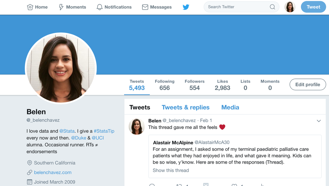
So I've decided it's time to clean up my Twitter feed. A start to my spring cleaning - online edition. While writing this post I Googled "Deleting old tweets" to see what came up regarding the topic and I came across a post on Digital Minimalism (the author deletes 40,000 old tweets). It was a fitting post, as it covers many of the reasons why I'm cleaning up my Twitter feed. For me, it's important to keep the online version of myself up-to-date and to be deliberate about what I post. (Though on the latter point, Twitter is more than anything a stream of consciousness social media platform so deliberateness doesn't quite apply.) Ultimately, by getting rid of my old tweets I'll be maintaining a fresher Twitter timeline. While on that Google search (deleting old tweets), I also found there are apps you can use to make your old tweets self-destruct after a certain number of hours/days. I'm not going to go into any of those. For this endeavor, I'll be using the Twitter API, Stata, and cURL to delete my old posts. Before I get started on deleting old tweets, this is what my Twitter profile looks like. Notice the 5,493 tweets, this is going to go down by the end of this post.
First things first, I downloaded my Twitter archive to get all of my tweets going back to the very first one - you can do this too by going to this link. Note that I didn't use the API since it can only return the most recent 3,200 tweets, for more information on the API check out Twitter's documentation.
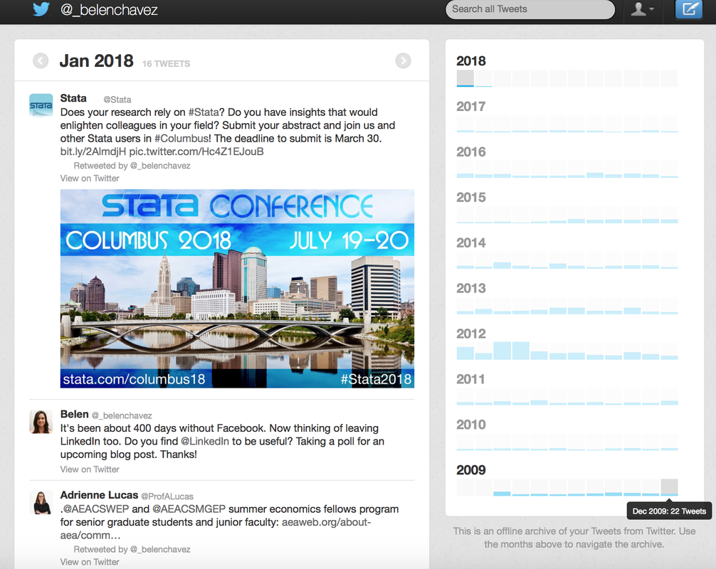
The downloaded archive includes my Twitter export (all tweet activity) in CSV and JSON format. There's also an archive browser interface where I can search through all tweets and browse tweets by year and month (right side of the image below). Mine looks like this:
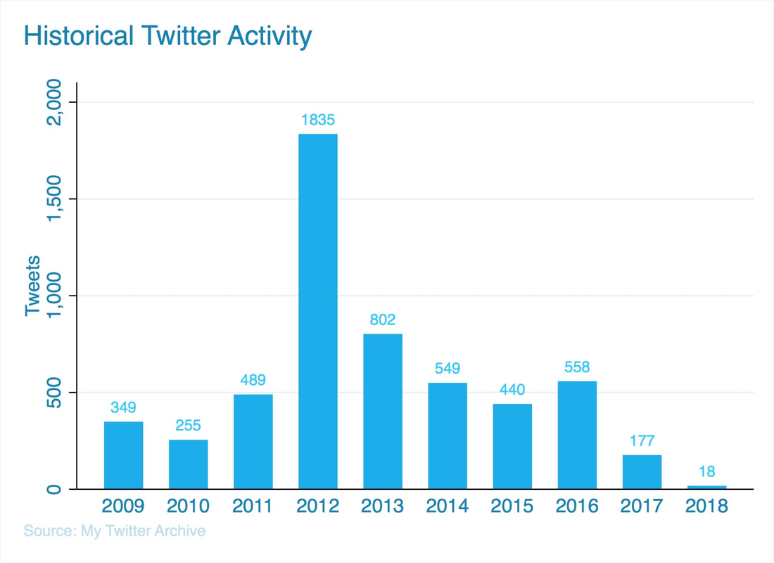
I imported my CSV file into Stata. Looking at my overall Twitter activity, I confirm that the bulk of my Twitter feed is indeed really old and outdated. About 80% of my tweets are from 2009-2014. I tweeted the most in 2012 and I tweeted the least last year. Here's a graph of my annual Twitter activity:
I made the bar graph using Stata and used Twitter's corresponding RGB colors. If you're interested in how I made it, here's the code for the graph:
graph bar totaltweets, over(year, label(labc("0 132 180"))) ///
        ylab(, labc("0 132 180")) blabel(total, c("29 202 255")) ///
        ytitl("Tweets", c("0 132 180")) bar(1, c("0  172 237"))///
        tit("Historical Twitter Activity",  c("0 132 180") span pos(11))  ///
        note("Source: My Twitter Archive", c("192 222 237") span) ///
        graphregion(color(white))
Now that I see what my activity looks like I can start flagging the tweets I want to delete. I'll be looping through the flagged tweets to delete them using the Twitter API. If you're not familiar with using Stata and the Twitter API together I suggest you first check out these two very informative blog posts by William Matsuoka: Stata and the Twitter API Part I and Part II, as I pretty much mirror his process.
First, I create a variable called delete which is equal to 1 if I want to delete that particular tweet (note: data is unique by tweet_id) Second, I decide what tweets I want to delete. My criteria is something like this:
In between the second and the third step, I also created another variable called always_keep that makes sure I keep Tweets with certain text in them like "Stata", "StataTip", "blogupdate", etc. This step is also not mentioned in the code below. As a short example, here's what my code looks for deleting tweets pre-2015:
clear all
set more off
version 15.1
/*Import the data*/
local twitter_dir "/Twitter API/Tweets/"
import delimited using "`twitter_dir'/twitter_archive/tweets.csv",  clear ///
     stringcols(1 2 3)  bindquotes(strict)
replace timestamp = subinstr(timestamp, "+0000","",.)
gen date = dofc(clock(timestamp,"YMDhms"))
/*Create variable to mark tweets I want to get rid of*/
gen delete = 1 if  year(date)<2015
levelsof tweet_id if delete ==1, local(mlist) clean
/*See http://www.wmatsuoka.com/stata/stata-and-the-twitter-api-part-ii
  for what's included in this following .do file */
qui do "`twitter_dir'/0-TWITTER-PROGRAMS.do"
* For Timestamp (oauth_timestamp) in GMT
/*Note: Will uses a plugin for this portion. I shelled out date program on my Mac */
tempfile f1
! date +%s > `f1'
mata: st_local("ts", cat("`f1'"))
/*Pass the timestamp and tweet_ids as arguments in the following loop*/
foreach tweetid in `mlist'{
        do 99_Delete_Tweets.do "`tweetid'" "`ts'"
}
The deletion of those pre-2015 tweets took my computer about 90 minutes to complete -- a rate of 40 tweets deleted per minute. The 99_Delete_Tweets.do file referenced above follows a very similar format to the one Will outlines in his blog post, except that instead of writing a tweet, we're removing it. For more information on deleting statuses see: Twitter's API Documentation. That do file looks a little something like this (note: I removed my personal API access information)
*99_Delete_Tweets.do:
*****************************************************************************
* Twitter API Access Keys
*****************************************************************************
* Consumer Key (oauth_consumer_key)
local cons_key = ""
* Consumer Secret
local cons_sec = ""
* Access Token
local accs_tok = ""
* Access Secret
local accs_sec = ""
* Signing Key
local s_key    = "`cons_sec'&`accs_sec'"
* Nonce (oauth_nonce)
mata: st_local("nonce", gen_nonce_32())
* Signature method (oauth_signature_method)
local sig_meth = "HMAC-SHA1"
*****************************************************************************
*Delete tweets
*****************************************************************************
local del_id   = "`1'"
local ts = "`2'"
* BASE URL
local b_url    = "https://api.twitter.com/1.1/statuses/destroy/`del_id'.json"
* Signature
mata: st_local("pe", percentencode("`b_url'"))
local sig = "oauth_consumer_key=`cons_key'&oauth_nonce=`nonce'&oauth_signature_method=HMAC-SHA1&oauth_timestamp=`ts'&oauth_token=`accs_tok'&oauth_version=1.0"
mata: st_local("pe_sig", percentencode("`sig'"))
local sig_base = "POST&`pe'&"
mata: x=sha1toascii(hmac_sha1("`s_key'", "`sig_base'`pe_sig'"))
mata: st_local("sig", percentencode(encode64(x)))
!curl -k --request "POST" "`b_url'" --header "Authorization: OAuth oauth_consumer_key="`cons_key'", oauth_nonce="`nonce'", oauth_signature="`sig'", oauth_signature_method="HMAC-SHA1", oauth_timestamp="`ts'", oauth_token="`accs_tok'", oauth_version="1.0"" --verbose
Having perused the remaining Tweets in my archive, I ended up deciding to discard tweets older than 90 days with the exception of those that I flagged as always_keep.
After all this, my Twitter timeline now consists of 210* tweets. So I got rid of 96% of my tweets. I imported my current Twitter timeline into Stata using twitter2stata, twitter2stata tweets _belenchavez, clear
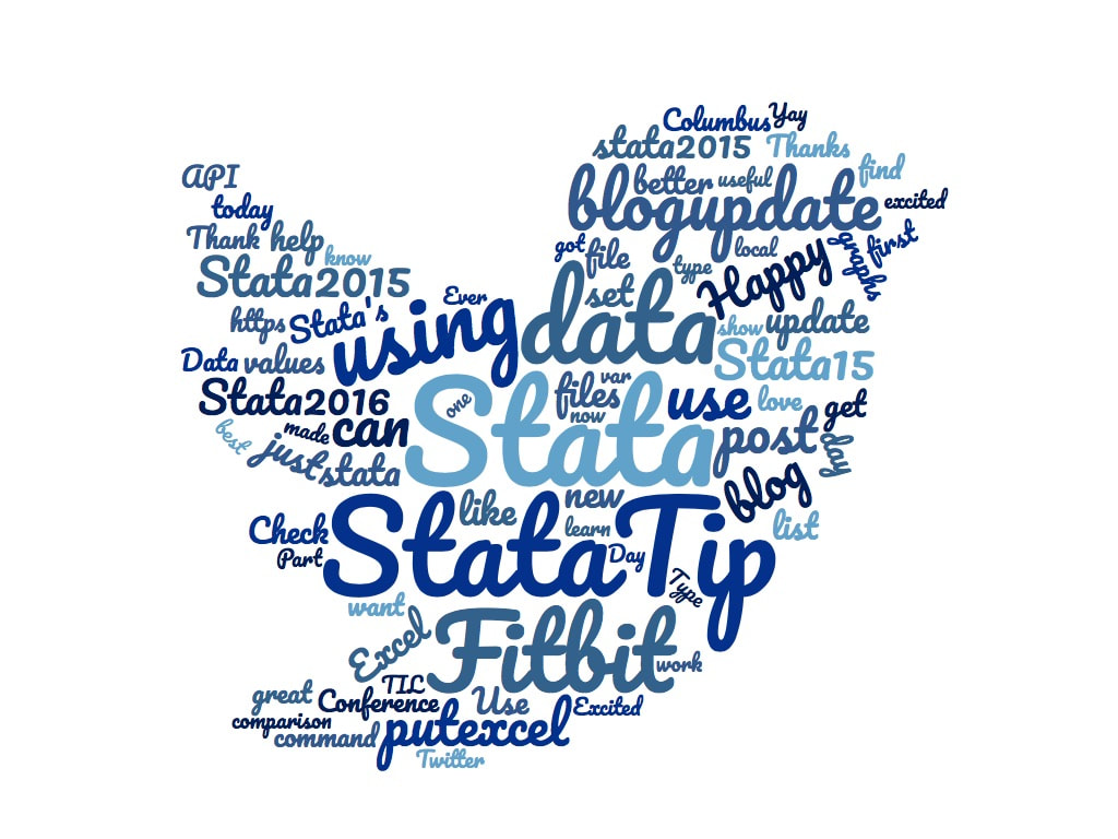
and created a visualization of my most commonly tweeted words using a word cloud. My new Twitter timeline is now up-to-date and fresher than before.
How many Stata's can you count?
Happy Anniversary, Twitter!
*Note: For as long as I can recall, I've had a discrepancy of 17 tweets on my timeline. So if you were to import my Twitter feed you'd get 193 tweets instead of the 210 that it shows me having on my Twitter profile. When users bulk delete their data there are 17 left over. It happens to a lot of people. The only recommendation I could find is to contact support.twitter.com.
0 Comments
Hello and Happy New Year, blog readers! I hope everyone's having a great 2018 so far. This month will mark the third year that I've had a Fitbit and you know what that means, right? I now have 3 years-worth of Fitbit data!
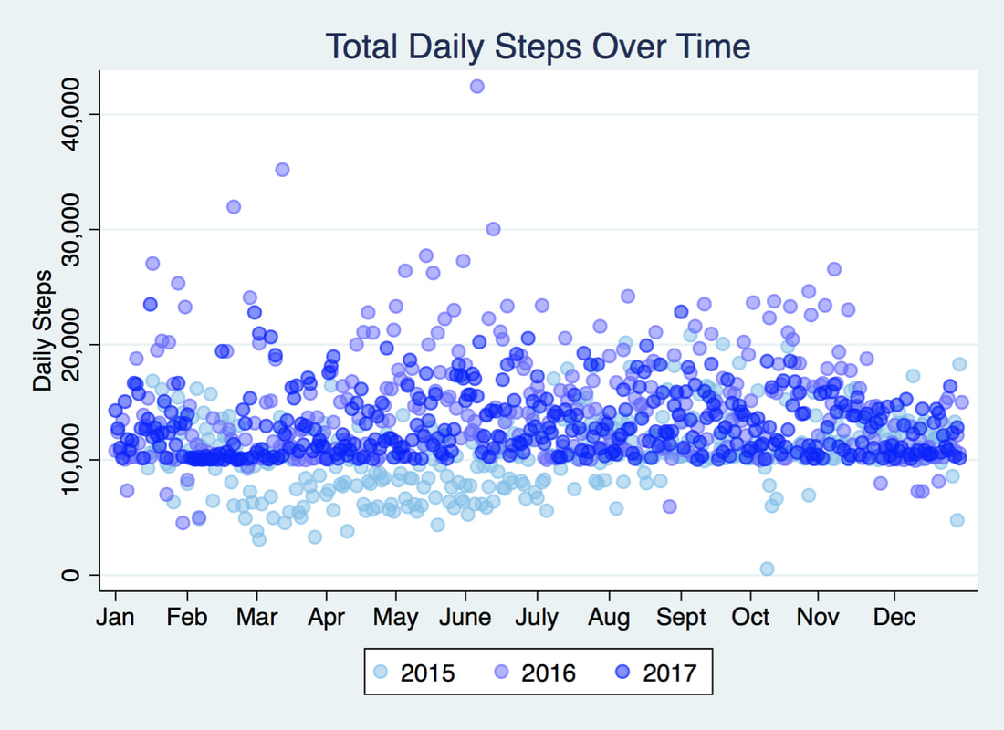
2017 was the first year where I met my step goal of 10,000 steps every single day. In fact, it's now been a solid 380 days since I last missed my goal. I intend on keeping this streak up in 2018. It should be noted that I participated in a Workweek Challenge with my Fitbit friends pretty much every week in 2017 which helped keep me accountable. Using Stata 15's newest graph transparency feature to plot my steps over the last 3 years you can see 2017 steps are consistently above 10k, though they're not as high as 2016's steps (as you'll recall, I trained for and ran 2 half marathons that year).
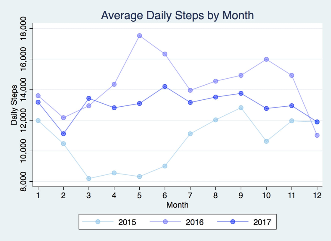
My steps in 2017 were fairly consistent with a range of 11k-14k average daily steps on a monthly basis. The chart below shows the average daily steps I took by month for each year that I've had my Fitbit:
Note that I don't have a full calendar year's worth of data for 2015 as my Fitbit arrived mid-January and it was stolen for a few days in October that year. Keeping that in mind here are the annual stats for each year that I've had my Fitbit:
Total steps taken: 2015: 3,695,222 2016: 5,257,825 2017: 4,747,316 Average steps taken per day: 2015: 10,528 2016: 14,366 2017: 13,006 My daily step maximum per year: 2015: 20,825 which happened on Sept. 6 2016: 42,431 which happened on June 5 2017: 23,503 which happened on Jan. 16 Number of days I missed my 10k daily step goal: 2015: 125 2016: 16 2017: 0 Using Google Charts, I've plotted the data below on a Calendar chart:
In the first 4 days of 2018 I've averaged 13,290 steps per day. It's also worth noting that I'm currently winning my Workweek Hustle as you can see in the small snippet below.
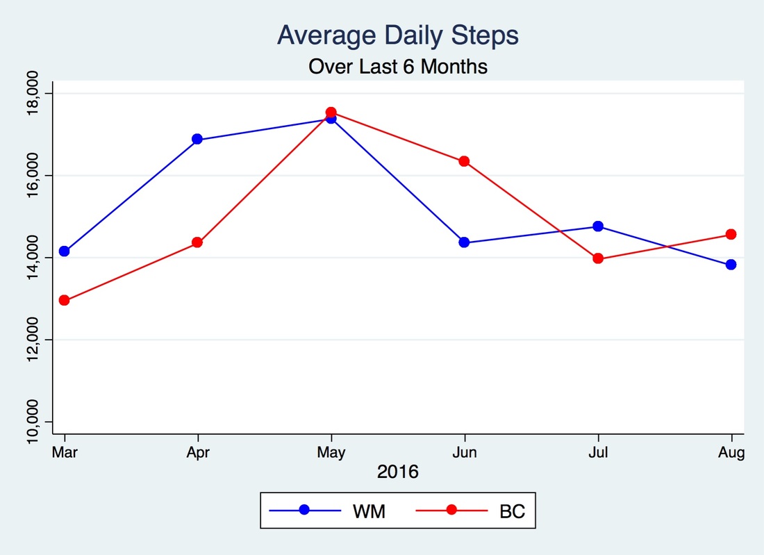
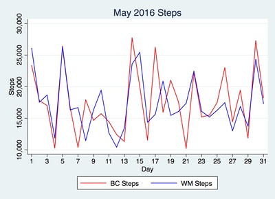
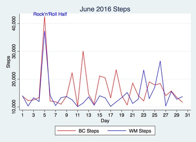
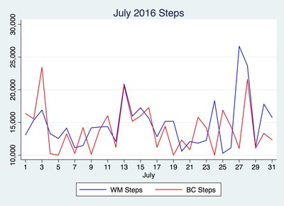
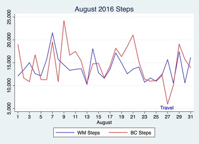
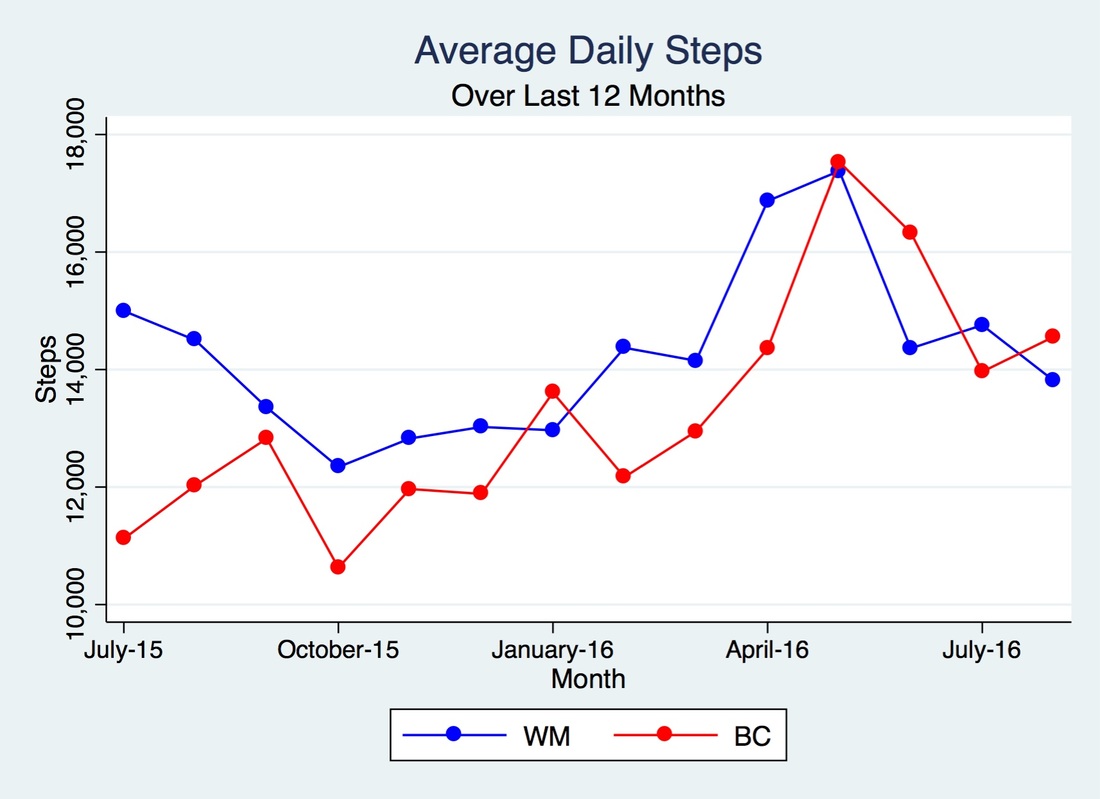
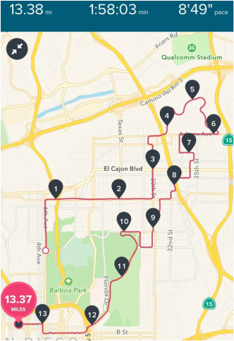
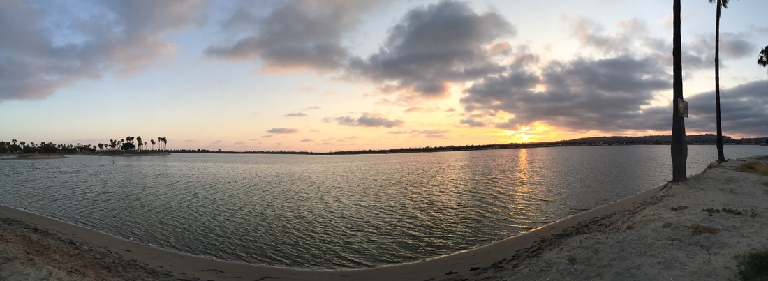
Cheers to 2018 and I hope this year's step counts are even better than last year's! Hello, again blog readers! It's been about 60 days since my last post and it's about time I did another Fitbit step comparison - the last one I did was in April. Yikes. Before I jump into that, let me take a minute to answer some questions you might have: What's new? Well, since I last blogged, a few things have happened. Like I went to Chicago to present at the Stata Conference and that was pretty awesome. I've never presented at a professional conference and our work was very well received. I got to visit San Diego a few weeks ago and that was very nice. We got to see old friends and hang out with family. I loved going back home. The beach was perfect, the weather was just right and the Mexican food was delicious. Besides that, work's good and time has gone by pretty fast. I can't believe I've been at my new job for 3 months. Seems like soon I won't be able to claim claim "new girl" status anymore. In Seattle, we've been exploring plenty of dog friendly places and we try to discover new places every weekend. Most recently, my blog was featured on Stata News! It felt so awesome seeing my name (with an accent and everything) and my blog post mentioned there. Thank you, Stata! For those of you who left a comment in that blog post, I will respond to it shortly. Why haven't I kept up with my blog? Not sure I have a good answer for that one - the easiest explanation is lack of free time. Any free time I do have I spend it with my fiancé and my dog, running, doing yoga/barre, or exploring the city. I will strive for more blog posts. Really. I like blogging, I like writing and I like exploring my data and sharing it with you all. You presented it and we you blogged about it, so where's gcharts? Yes, I presented beta version at the conference. Will and I are working on it and hope to have it ready for public release in the next few weeks. Stay tuned. If you have any additional questions, feel free to ask away. Okay, now moving onto the blog post. So what has my steps data looked like from May to now? This is especially interesting as I did another half marathon in June and moved soon after. My schedule, work, and day to day activities have changed a lot since moving from San Diego. Below you'll see my average daily steps for the last 6 months compared to my friend Will's average daily steps. Interestingly, our steps show a similar trend leading up to and right after May 2016. May was my last full month in San Diego, so my hypothesis is that the decrease in joint work break walks and half-marathon training has something to do with that decrease for the both of us. Keeping with the tradition of posting monthly graphs, I've graphed our daily step activity for May through August below. As I mentioned earlier, Will and I ran the Rock'n'Roll Half on June 5th in San Diego which explains that spike. That date also happens to coincide with the personal record, in terms of daily steps (42,431 steps) and half-marathon finish time, of your's truly. 1:58:32. I know! Thank you. Not bad for my second half. Although, I must say that course was a lot easier than my first one. I also moved to Seattle in June and unfortunately for Will, the asphalt around Balboa Park was pretty bad so and he tripped and scraped his knees and palms around mile 8 or 9 of the course (he needed stitches) and so those injuries are the reason for his low step count that month. July is interesting in that there are a few days with very similar steps. A group of us, including Will, had Fitbit challenges (Work Week Hustle and Weekend Warrior Challenges - these are challenges through the app where you compete with friends in total steps during weekdays and weekends. More on that in a post to follow) and so I'm thinking that's why there are a lot of days with similar step activity, not sure though. I'll have to look into that and get back to you. August is funny. I didn't meet goal on a Saturday during my vacation! I tried, people, but Orange County is not that close to San Diego (traffic took a while) and lounging on the beach doesn't allow for many steps. Oh well, at least I had fun in the sun, and isn't that the point? Overall, August was a pretty good month for steps. Below, I've graphed our average hourly step count during weekdays (I also excluded holidays). I wanted to see what our graphs looked like together before and after I moved and I'm using Will's hourly step shape as a control. This data represents 60 days before and 60 days after moving. Interestingly, our hourly weekday graphs are very similar when I was in SD (March - May) and are not so similar when I moved (June-August). The similarity of our hourly graphs is due to the similarity in work schedules, meetings, lunch breaks, etc. Both of our hourly shapes changed after I moved. For me, the reason is that I walk more now that I don't drive to work and I'm allowed to bring my dog to the office so there's that difference, too. I take a couple of dog walks (about 2 a day, though, so not that many) 2-3 times a week. For Will, I'm not sure what's changed in his day-to-day, so you'll have to call and ask him. My speculation is now that our other friends/coworkers also have Fitbits/Garmin trackers maybe they take walks at different times. I'll find out. Now that I've updated you on the last few months of Fitbit activity, I thought it appropriate to look at the last year just to see what that all looks like. That's July 2015 - August 2016 average daily steps for the both of us. Cool, right? While, I only beat Will's average daily step count 4 out of 13 months, you can see how positive of an effect training for both half marathons had on our step activity. I'm tempted to sign up for another one soon, but it should definitely be held someplace warm. It's already cooling down over here and running outside is hard for this Southern Californian. Well, there you have it. I hope you've enjoyed this latest blog post. I'll leave you with this cool picture of my Rock'N'Roll race course graph as seen through my Fitbit app. I loved saying farewell to my favorite city by running through some of my favorite parts of it. In case you're wondering, Mission Bay is my absolute favorite running spot in San Diego. And just so you know what I'm talking about, here's a picture I took of Mission Bay on my last sunset run there. I know this isn't Instagram, so this should go without saying, but no filter was used to touch this picture up. Gorgeous, right? Until next time, blog readers.
Recently, I assigned a GIS problem set to my students and had them geocode addresses to obtain latitude and longitude coordinates using mqgeocode in Stata. The reason I had them use mqgeocode and not geocode3 is because the latter is no longer available through ssc. Does anybody know why? Somebody please tell me. What's the difference between the two? One difference between the two is that mqgeocode uses MapQuest API and geocode3 uses Google Geocoding API.
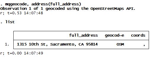
Anyway, after my students downloaded mqgeocode, I received several emails from students letting me know that they could not obtain coordinates no matter what format the addresses were in. See below:
What? No coords? Why not? With the help of the nice people over at www.wmatsuoka.com we dug a little deeper and saw that the API key in that program had probably hit its limit which is why it wasn't returning any coordinates.
A quick fix for that is to replace the two lines in that ado file with your personal API key. How do you get a MapQuest API key? Just sign up for one here. It's pretty quick and fairly easy. Then look for the lines "local osm_url1 =" and put in your own API key. I put in my API key in a local called `apikey' which was passed on to the following lines in that program. The following two lines correspond to lines 47 and 141 of the mqgeocode.ado file, respectively:
local osm_url1 = "http://open.mapquestapi.com/geocoding/v1/reverse?key=`apikey'&location="

local osm_url1 = "http://open.mapquestapi.com/geocoding/v1/address?key=`apikey'&location="
I renamed that ado file and program as mqgeo2 and quickly got to geocoding:
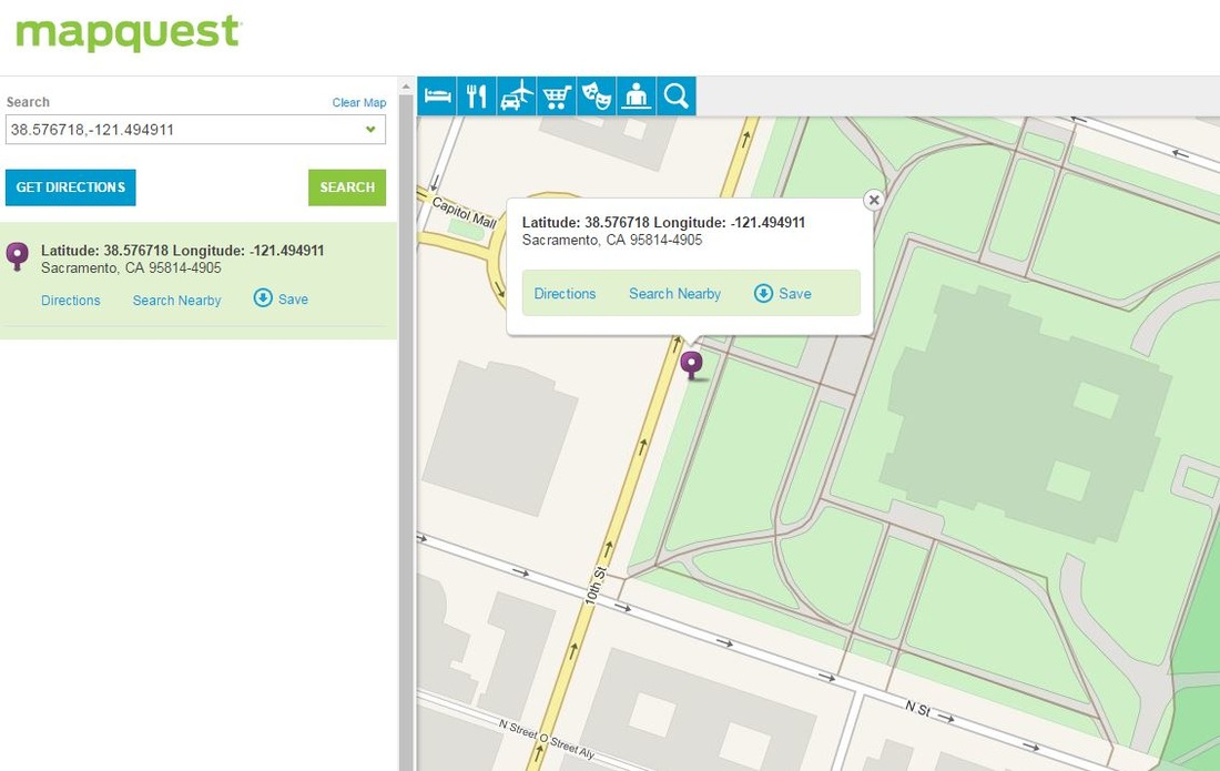
And voilà! We now have latitude and longitude coordinates for our address which happens to be the California State Capitol building.
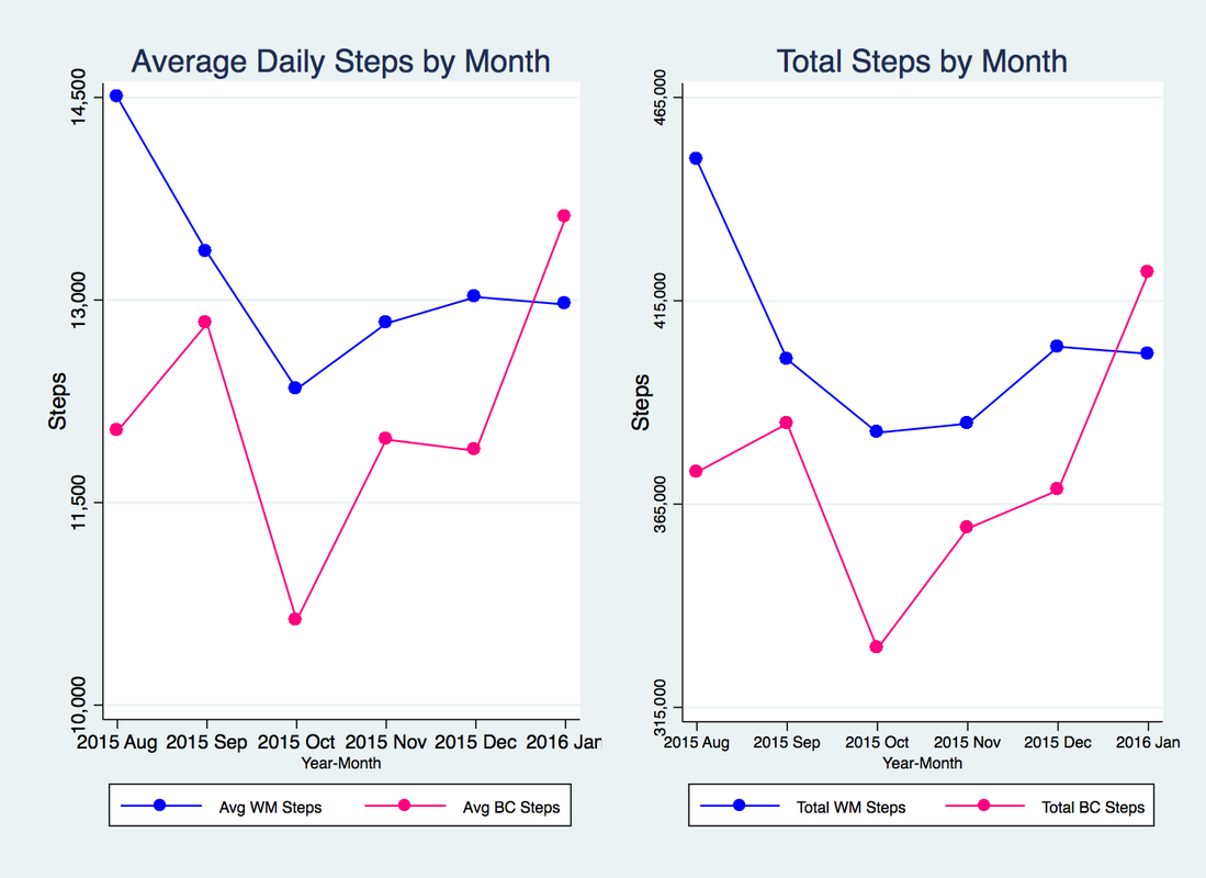
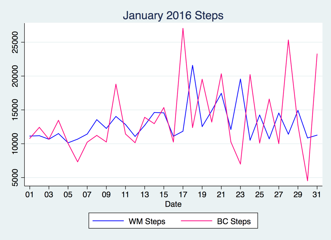
Ta da! This is what (old) MapQuest looks like (I miss Google already) I am proud to say that my half-marathon training has increased my step count. January 2016 has been my best month yet. Totally patting myself on the back. Below I've graphed my average daily step count and my total monthly step count and comparing it to Will's for the last 6 months. Recall that I had my Fitbit stolen in October which is why there's a dip in October 2015. My average daily steps in January: 13,608 versus Will's 12,966. My total monthly steps in January: 421,858 versus Will's 401,965. I had a 14.5% increase in activity from December to January. While Will had a minuscule drop in step activity (about -0.4% change). Below is what the daily step counts looked like. The spike on the 17th is my personal record for most daily steps. It also beats Will's daily record of 25,370 steps. I got 27,026 steps that day. Note that in 2015, my daily step record was 20,825. In January 2016 I managed to get above 20,000 steps 5 times. (I only got above 20,000 steps 3 times in 2015). Hooray for running and training! In the last couple of weeks I've slowed down on my training due to a bug I caught, but I'll be running again soon. Stay tuned for February's update next month :)
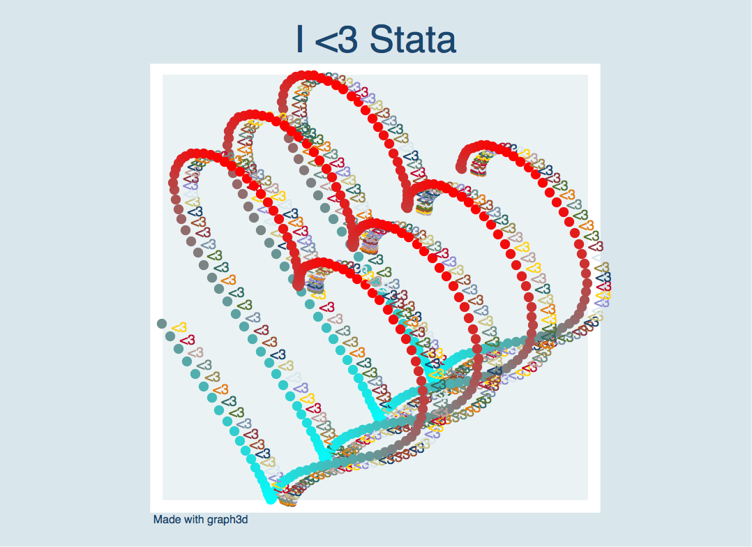
Happy Valentine's Day! Combine today with Stata and you get a heart shaped graph. The one I made below was made using graph3d in Stata.
Did you notice I also used the "<3" marker labels here? Hearts on hearts on this graph ;)
Below is the code I used to make the heart graph. I added the title, note, and other options using the graph editor.
/* Author: Belen Chavez
     Stata Heart Code
     Happy Valentine's Day <3 */

clear all
set obs 463
gen t = .
local c = 1
forv i = 0(0.05)`=2`c(pi)''{
        replace t = `i' in `c'
        local ++c
}

gen x = 16*sin(t)^3
gen y = 13*cos(t)-5*cos(2*t)-2*cos(3*t)-cos(4*t)
gen mlab = "<3"
graph3d x y t , colorscheme(cr) scale(3) markeroptions(mlab(mlab))
Happy Valentine's Day to my blog readers <3
A few days ago, I attended the San Diego Economic Roundtable at the University of San Diego which included a panel of experts discussing the economic outlook for San Diego County. My favorite speakers were Marc Martin, VP of Beer, from Karl Strauss and Navrina Singh, Director Product Management, from Qualcomm. Singh had a lot to say about data, technology, innovation and start ups in San Diego County. Did you know that there are 27 coworking spaces, accelerators, and incubators in San Diego? I sure didn't. Martin's discussion of beer, all the data he showed, along with some cool maps, sparked this blog post which has been a long time coming. In case you don't know, I'm quite the craft beer enthusiast! Allow me to nerd out as two of my favorite things come together: data and craft beer.
Martin's talk focused on the growing number of microbreweries and craft beer data. Here are some cool facts I came away with from his presentation that are worth mentioning again:
On to my blog post: While searching for beer data for this blog post, I stumbled across a gold mine: BreweryDB.com. I got access to their data using API. In the last few days, I've looped through over 750 requests using Stata's shell command and Will's helpful post on Stata & cURL. In the table below I've detailed the number of beers (listed as results) under each style ID in BreweryDB's database. There are a total of 48,841 beers as of January 17, 2016. When filtering for the word "Belgian" in the style name, I got a total of 5,883 beers. Can you guess what my favorite type of beer is? :) I made the table below using Google Charts API table visualization. There are a total of 170 beer style IDs under BreweryDB and I've summed up the number of beers under each style. You can sort by ID, Beer Style or Results by clicking on whichever column title you'd like.
Disclaimer: This product uses the BreweryDB API but is not endorsed or certified by PintLabs.
Seeing as BreweryDB's data is extensive and I'm oh-so excited to share with you some of my findings, I've decided to make a series of blog posts about this. This is why this is part 1. This is only the tip of the iceberg, my friends, and I'm not sure how big of an iceberg I'll be uncovering, but stay tuned for more.
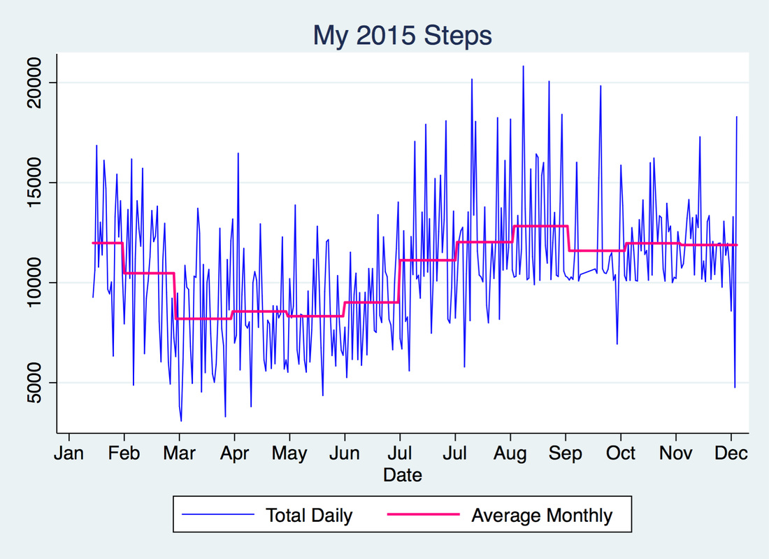
I got my Fitbit on January 15, 2015 and I have been obsessed with it ever since (sorry not sorry, friends and family). I figured that now that 2015 is over, I'd look at my step trends for the year. The graph above shows my total daily steps in blue and my average monthly steps in pink. As you can see, my average daily steps went up after July and remained above 10k throughout the end of the year.
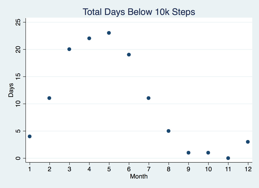
I wasn't meeting goal very often before July and this is evidenced in the graph below. It counts how many times I missed my step goal for every month in 2015:
I got better at meeting goal and became more competitive as more people I knew (like Will) got Fitbits and challenged me with Fitbit's Goal Day, Weekend Warrior, Daily Showdown and Workweek Hustle challenges.
Using Stata and Google Charts API I made the following graphic which shows my steps above or below my goal of 10k.
This was motivated by my Fitbit & Google Calendar Chart blog post. The legend is similar:
This includes a total of 344 days. My average daily steps for 2015 was 10,593 steps, and for the months of July through December was 11,910. Also, as the Stata graphs above illustrate, the months of February through June show a lot of days where I missed my step goal. For 2016, I'm aiming to have a lot more blue cells with darker shades of blue. That's my resolution :)
I was playing around with some Google Charts yesterday and I stumbled across their Calendar charts. I thought it would be cool to display changes in Fitbit activity by displaying step differentials using this visualization.
The legend is as follows:
The chart above shows 145 days of data with varying levels of competition. Unfortunately for me, there are mostly blue cells. Will's a runner, so unfair advantage, right? With the exception of September, I beat Will's step count for a total of 7-8 days out of the month. In September I beat his step count for a total of 14 days. Still, that was only 46% of the days in July. Go Will! He takes the lead 75% of the time. You can see the cell colors becoming lighter from July to November. In other words, the step counts were converging, meaning 1 of 2 things: 1) We got more competitive, or 2) we both got less competitive as time went on. See for yourself below:
Looks like a slight downward trend from August to November.
These cool charts were made in Stata and use Google Charts API :)
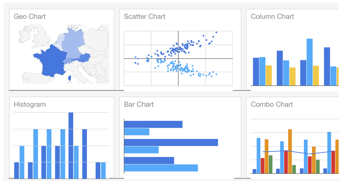
Not long ago, I was introduced to Google Charts. Ever since, I've been obsessed. I now love using Stata and combining it with Google Charts. Step 1: Clean data using Stata, Step 2: present data using Google Charts. Result: Easy to read and aesthetically pleasing visualizations for my website. Perfect.
Last month, I scraped Hayek's instagram data and made a paw-some map from the extracted latitude/longitude pairs using Google Charts and an .ado file that I came across thanks to Will, written by a former coworker of his called gmapmark which writes an .html file that creates a Google map. See said map in my dog blog: http://www.belenchavez.com/hayek/dog-friendly-sd
I decided to improve that program by incorporating the ability to have different markers for the data points by using web addresses that point to .png, .gif or .jpg images (like I did for the paw prints above). I've also added the ability to name your data points, instead of simply showing the latitude/longitude information. I've called that program gcmap short for Google Charts map. For more on making map visualizations check out Google Charts.
Example 1:
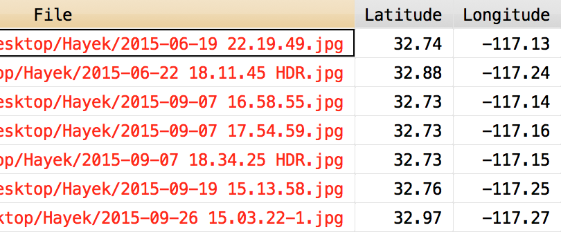
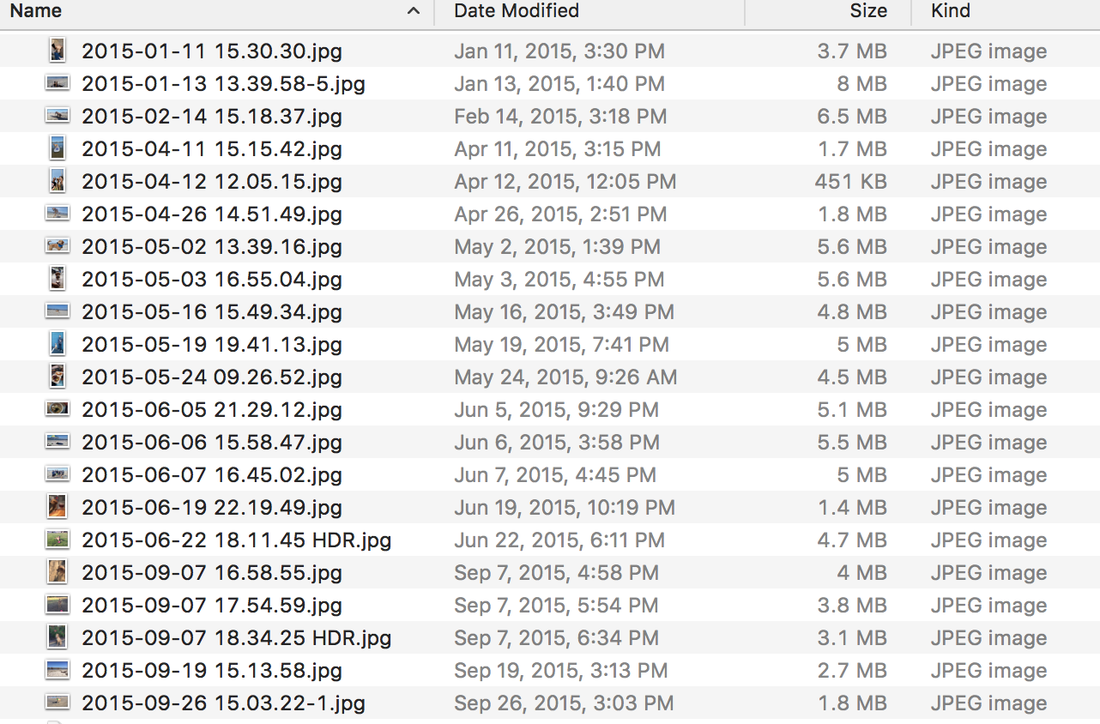
Do you own an iPhone? Do you use Photos? While I do use the Photos app on my phone, I don't like it on my computer, so I keep a separate folder of uploaded pictures that Photos doesn't touch. Back to the point, one of the features that Photos has is the ability to make a map of your pictures if your pictures have location information. Did you know that we can also make such a map using Stata and Google maps? You didn't? Well, now you know :) Let's say I want to make a Google map from several pictures I have in a folder called Hayek. How do I do that? Well first, I will extract the latitude and longitude information using exiflatlon that I have thanks to Will's post on exif information. clear version 12.1 cd Hayek exiflatlon, dir() clear * Exclude files missing lat/long data drop in 1/14
This makes the following dataset with latitude and latitude information from exif data in the pictures contained in the following folder:
I type the following into Stata after downloading gcmap and placing it in my personal ado folder. In the following example, I want the name() of the data points to be the file names from above contained in the variable "File". The option nor() contains the web location of the icon to display for the data points, which is short for normark(). The sel() option contains the web location of the icon I want to use for once a data point is selected on the map, it's short for selmark().
gcmap using "hayek_paws.html", latitude(Lat) longitude(Lon) name(File) ///
        zoom(11) ///
        nor(http://www.belenchavez.com/uploads/5/6/9/3/56930511/9243470_orig.png) ///
        sel(http://www.belenchavez.com/uploads/5/6/9/3/56930511/5261019_orig.png) ///
        replace
Which makes the following map:
Note: I could have left the nor() and the sel() options empty and this would have made a map with the usual red balloon marker points. See example below.
Example 2: I can also make a Google map from the Google location history data I have for a couple of days back in October and use the time stamp as the name for each point. Here, I don't specify nor() or sel(), so the default map markers show up. gcmap using "trip.html", lat(latitudeE7) long(longitudeE7) name(tstamp)
And there you have it! Now you too can use gcmap to make cool Google maps using Stata. Easy, right?
|
AuthorMy name is Belen, I like to play with data using Stata during work hours and in my free time. I like blogging about my Fitbit, Stata, and random musings. Archives
March 2018
Categories
All
|
||||||||||||
